Do you love data? If you do, then you need to read our R tutorial for data science.

Data science is an important tool for understanding complex data sets. Without data science, we will not be able to make sense of data.

That’s why, today, we will go through the R tutorial for data science. 

The tutorial will be a complete guide on using R with data science. If you are a beginner, you can gain a lot of knowledge by going through the article. 

So, without any delay, let’s get started with it already.

R tutorial for data science

R is a programming language that is not developed by software developers or programmers but is developed by a data scientist for working with data.

It was first released in the 90s, and it has grown in popularity and usage among the data science enthusiasts.

R is an excellent pick for data enthusiast as it enables them to save scripts. It allows you to generate reproducible work. Also, R works on all the major operating systems, including Linux, Windows, and Mac OS.

Why learn R?

There are many benefits of using the R programming language. 

The ecosystem of R is mature. You can install library and packages that are developed and maintained by other R developers and users.

The interactive console is at the core of R software. You can do small calculations using it. However, the ability to create scripts make it more appealing to learners and enthusiasts

There are many advantages of using R. Let’s list them below.

• Open source and free to use
• Save scripts for reproducible work
• Tons of online resources to learn and explore data science through R
• Share software implementation easily
• Easy to install
• Coding style is easy
• Great community support. 
• R is a highly sought skill in the industry
• More than 7800 packages to explore and use
• Supports high performance computing experience

How to install R

As R is free software, you can install it on your computer without any trouble.

To get started, you need to download go to the Comprehensive R Archive Network. From there, you can download the version according to your OS.

For the tutorial, we will be using Windows 10 OS.

Once R is installed, you now need to install R Studio.

R Studio offers a more compact and fluent experience while working with the R programming language.

RStudio is an integrated development environment(IDE). You can download it from the RStudio website. Choose the “free” version.

Also read, Google’s Go Programming Language Is Going Places—By How Far?

RStudio Interface explanation

RStudio can seem a little complicated for beginners. To ensure that you do not have confusion, let’s go through the key interface elements below.

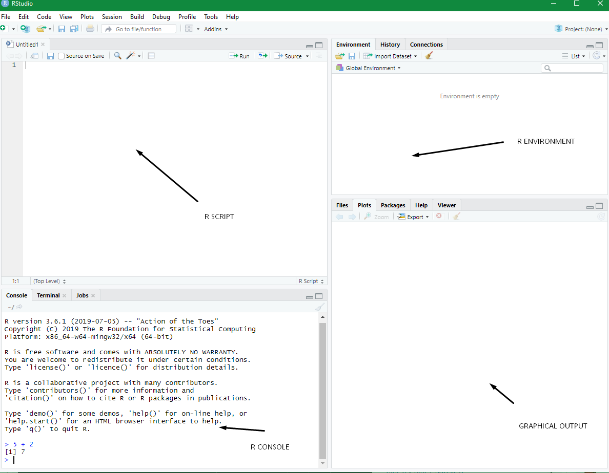
• R Script: This is the area where you will write your code.
• R Console: Here, you get to see the output of your code. The code can be run by selecting it and pressing Ctrl + Enter.
• R Environment: The R environment is the section where you get information about your code. It can include variables, data set, functions, and so on. It also shows other vital information
• Graphical Output: The area is dedicated to showing the graphical outcome of your script and data.

Installing R Packages

R is a programming language and acts as a tool. However, its library is what makes it more useful. In this section, we will be learning how to install R packages. These R packages have specific purposes and can be loaded directly from the console.

To install a specific package, you need to do the following:

If you type the above command correctly, you will get a popup to choose the CRAN mirror from where you can want to download the package. You can select the CRAN mirror to your country or near to your country. Once done, the installation will begin.

R Basics

With all the necessary tools and IDE installed, it is now time to get started with R.

R programming language is easy to get started with. 

You can do basic computations by typing the following in the console.

R Basic Computation

In the above code, the > is where you input a statement. The output is marked by [1]

You can do the basic computations using R. Moreover, you can also access the old executed commands by pressing the up or down arrow key.

R Variables

Variables let you store information in memory. Variables can also be referenced later on. 

In R, you can assign a value to a variable by using the <- or the = sign.

The following code assigns 1 in variable a.

In the above code, we stored value of 1 in variable a.

To see the value stored in a, you need to enter “a” in the console. You can also use the print(variable-name) to see the store value.

Objects

An object is defined as the values that are stored in R. Objects can be as simple as a number or a complex function.

Obviously, you can access what’s within the object by calling them in the console. 

To know what objects are currently defined in the workspace, you can use the ls() function.

Workspace is created when you start working in RStudio.

If we had more variables stored in the workspace, it would have listed them as well.

Also, if you try to refer to an object which is not defined, it will throw the following message.

Functions

Data analysis is all about applying functions to stored data. For example, you can store 64 in “a” variable and then run sqrt() function over it.

As usual, you get eight returned to the console.

Libraries offer a vast range of functions at your disposal. This makes your work easier so that you can focus on the task at hand rather than reinventing the wheel.

R already comes with a predefined set of functions, similar to the sqrt() function.

To learn about them, you need to open up the documentation and go through it. The console or the workspace doesn’t list the functions which can leave you stuck in a few occasions.

The syntax in the case of functions is important. Without parentheses, the function name will return the code itself.

It can help you learn how the code works behind the scenes. However, to make the function as intended, you need to use parenthesis() to the function name.

It returns the log on 100.

Moreover, if a function takes an argument, then you need to specify it beforehand. If not done properly, it can show the following error.

Functions also work with variables.

This comes handy when you are writing big programs that take different variables.

If you are not sure what a function does, you can use the function help() to learn about it. The help systems are beneficial, which provides you valuable information.

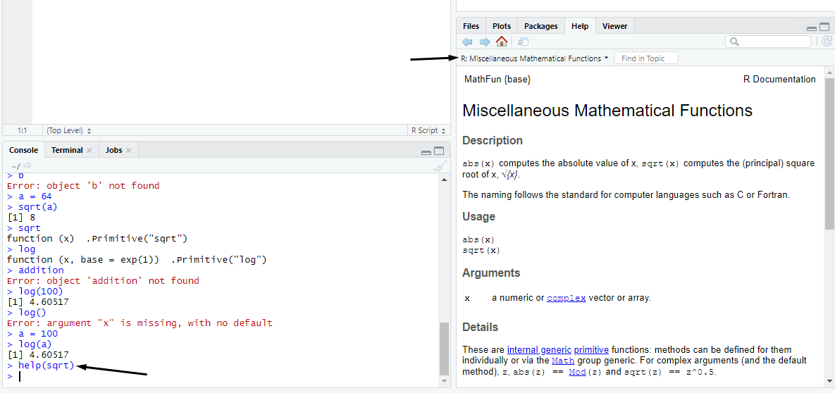
To know what arguments a function takes, you can type the args() function.

You can also type log(9,3), and it will still return 2. The R editor understands what the three stands for, and hence you do not have to type base.

Datasets

Just like functions, you can also check out the datasets. Datasets are built in R. You can check it out by typing data().

You can use these object names that contain the data.

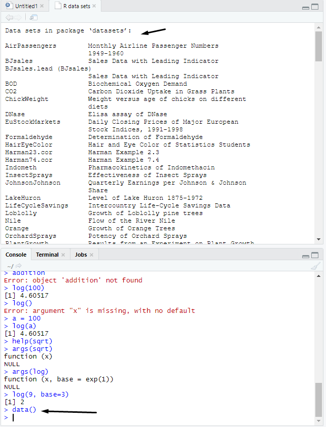
You can further check the data stored in these dataset objects by typing the object name in the console.

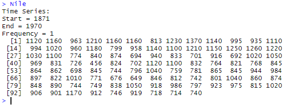
The above dataset is from the river Nile. 

Lastly, you need to be aware of the variable names correctly. There are many rules that you need to follow while naming the variables.

• Variable name should start from a letter
• Should not contain spaces
• The variable name should not match function or dataset defined in R.

Scripts

Writing a script is more useful in the long run. It adds value to your work as you can use it later on. You can create scripts and use in your larger projects. 

Also, breaking your program into scripts can help you in the long run. You should also want to comment your code so that you can understand the purpose later on while editing the code. Other coders can also understand the intent by reading the comments.

Learning About Data Types

Now, that we have covered the basics of R, it is time to dive deep into the R tutorial. In this R tutorial, it is essential to learn about data types.

The values stored in the object can be of different types. The type depends on the nature of the value stored in the object.

To know which data type the object is storing, you can use the class() function.

As you can see from the above code, if we store value 1 in “a,” and then enquire about the datatype of “a.” As you can see, it returns, “numeric.”

Similarly, you can find out the class of other data types. Let’s check out the following code.

The above is a character data type. 

In R, there are five types of objects.

• Numeric e.g., 1.2,2.3 etc. (real numbers)
• Character e.g., “a”, “moon” (names and alphabets)
• Complex, e.g.,  
• Integer, e.g., 1, 9, 5 (whole numbers)
• Logical, e.g., (true, false)

Data Frames

As a data scientist, you will be using data frames. They are the most used way of storing information and are the synonym of tables. The columns represent the variables, whereas the rows represent the observations.

But, if you want to know more about the structure of the data frame or the object within a data frame, then you can str() function.

The str() function shows the structure of the data.

As we already know that there are many datasets present within R. To get started, let’s check out the head of the CO2. It will show only the first few rows within the data object.

Here you can see the variables in the rows. The variables for CO2, you can see variables such as Plant, Type, Treatment, Conc, and Uptake. Each row shows the data stored against the variables in the columns. 

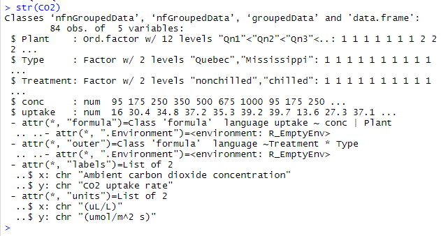
Accessing the variables: To access the variables, you can use the $ symbol. Let’s do it below. It shows all the data associated with the column.

To know the names of the variables associated with an object, you can use the names() function.

Vectors

This leads us to vectors. Vectors can contain one or more value from a particular object of the same class. So, for example, the CO2$uptake is a vector that includes a range of numeric values.

You can play with these vectors and can find information about them.

Similarly, you can also have a character vector. Character vector contains a string.

CO2$ Type will return a character vector which consists of the Type of plants that release CO2.

Also, you need to use quotes if you need to store a character.

We also have a logical vector that store value of either True or False.

We will dive deep into vectors.

Creating a vector is easy. All you need to use the concatenate function.

You can also associate the name to each of the value. For example, you can do the following to store information in a vector.

You can also create a sequence function to generate the vector. This is very useful to generate a list.

To access the element, you need to use [].

For example, you can use num[2], and it will return 212.

Similarly, you can also access a certain part of your vector by using the following code:

You can even access it by ab[first], and it will return a value of 200

Vector Coercion: Vectors work differently in R. We need to understand how it works as it can help you understand the behavior of R.

As you can see in the above example, if we decide to allocate a string and two numbers in “y” vector, we get a vector that only contains characters.

R transforms the vector based on the fact that it can change the data type of numbers to characters and not the other way around.

If you check the class of “y,” you will get the following answer.

Similarly, you can change numbers to characters using the “as” numeric function.

Similarly, if the coercion process fails, it will throw NA. This happens when you try to change the character to number.

Factors

Factors is another exciting type of data type. It is used to store categorical data. Many data is categorized and storing the data this way can help with memory-efficient storage.

This is how you convert any vector into factor data so that you can store categorical data.

R Control Structures

Let’s move into the R control structures in our R tutorial. Control structures are useful to manage our commands within a particular function.

It also helps you to take care of any repetitive task until a condition is met. This way, you can write less code and get your work done pretty fast.

Let’s look first at if-else.

In if-else, the code below “if” is executed if the condition is met, otherwise the code below “else” is executed.

If (condition) {do this}

else {do this one instead}

The “for” loop is used to go through a particular code until the exit condition is met.

for (check if condition is right or not) {

Execute this;

}

You can also use while loop which works like below:

while(condition) {do this}

This leads us to the end of our R tutorial basics for data science. Now, let’s move on to some advanced stuff including packages and working with a data set.

Conclusion

This leads us to the end of the part of the R tutorial for data science series. In part 2, we will cover more important concepts about R and how they can be utilized in data science.

So, stay tuned for the next part!